Clusterpolate

Inter- and Extrapolation for Scattered Data

Traditional approaches for inter- and extrapolation of scattered data work on a filled rectangular area surrounding the data points or in their filled convex hull. However, scattered data often consists of different clusters of irregular shapes and usually contains areas where there simply is no data. Forcing such data into a traditional inter- or extrapolation scheme often does not lead to the desired results.

Heatmaps, on the other hand, deal well with scattered data but often do not provide real interpolation: Instead they usually use raw sums of kernel functions which overestimate the target value in densely populated areas.

Clusterpolation is a hybrid inter- and extrapolation scheme to fix this. It uses kernel functions for a weighted inter- and extrapolation of local values, as well as for a density estimation of the data. The latter is used to assign a membership degree to clusterpolated points: Points with a low membership degree lie in an area where there’s just not enough data.

Installation

The clusterpolate package is available from PyPI and can be installed via pip:

pip install clusterpolate

Quickstart

Use image() to generate images using clusterpolated data:

import numpy as np
from matplotlib.cm import summer
import matplotlib.pyplot as plt
from clusterpolate import image

# Generate some data
n = 500
angles = np.random.normal(0, 0.75, n) - 0.2 * np.pi
radii = np.random.normal(1, 0.05, n)
points = np.vstack((radii * np.sin(angles),
                   radii * np.cos(angles))).T
values = np.sin(angles) + np.random.normal(0, 0.5, n)
size = (500, 500)
area = ((-1.5, 1.5), (1.5, -1.5))

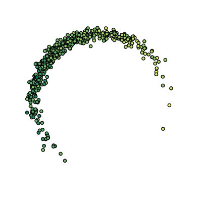
# Plot raw data
plt.scatter(points[:, 0], points[:, 1], c=values, cmap='summer')
plt.axis('equal')
plt.axis([-1.5, 1.5, -1.5, 1.5])
plt.gca().set_aspect('equal', adjustable='box')
plt.axis('off')
plt.show()

# Generate clusterpolated image
img = image(points, values, size, area, radius=0.2,
            colormap=summer)[3]
img.save('clusterpolated.png')

Raw data:

Clusterpolated data:

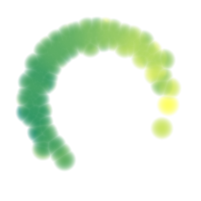
Note how the values are cleanly interpolated even within dense regions and how extrapolation only occurs close to existing data points.

Of course you can also use clusterpolation on your data without generating any images: simply use clusterpolate().

API Reference

clusterpolate.bounding_box(points)

Compute a point cloud’s bounding box.

points is a list or array of 2D points.

The return value is a 2x2 tuple containing the upper left and the lower right bounding box corners.

clusterpolate.bump(r)

Factory for bump kernel functions.

r is the radius of the bump function.

The returned bump function assumes that all values in the input vector are non-negative.

clusterpolate.clusterpolate(points, values, targets, radius=1, kernel_factory=<function bump>, neighbors=None, num_jobs=None)

Clusterpolate data.

points (array-like) are the data points and values (array-like) are the associated values. targets (array-like) are the points at which the data should be clusterpolated.

radius (float) is the radius of each data point’s kernel.

kernel_factory is a function that takes a radius and returns a corresponding kernel function. The kernel function must accept an array of distances (>= 0) and return the corresponding kernel values. The kernel function must be normalized (a distance of 0 must yield a value of 1) and it should be zero for distances greater than radius.

Neighbor lookup is done using an instance of sklearn.neighbors.NearestNeighbors, constructed with the default options. You can pass an instance that is configured to suit your data via the neighbors parameter.

By default, computations are parallelized according to the number of available CPUs. Set num_jobs to a specific number to use more or fewer parallel processes.

Returns two arrays. The first contains the predicted value for the corresponding target point, and the second contains the target point’s degree of membership (a float between 0 and 1).

clusterpolate.image(points, values, size, area=None, normalize=True, colormap=None, **kwargs)

Create an image for clusterpolated data.

points and values is the input data, see clusterpolate().

size is a 2-tuple containing the image dimensions.

area is an optional 2-tuple of 2-tuples, specifying the top-left and bottom-right corner of the sampling area. If it is not given then the points’ bounding box is used.

If normalize is true then the clusterpolated values are normalized to the range [0, 1]. If you set this to False you should ensure that input values are already in that range.

colormap is an optional callback that can be used to color the clusterpolated values. It should accept values in a 2D array and return the corresponding colors in an array of the same shape but with an extra dimension containing the RGB components (between 0 and 1). The colormaps from matplotlib.cm are a good choice. If no colormap is given then a grayscale image is generated.

Any additional keyword-argument is passed on to clusterpolate().

This function returns 4 values: The first 3 are arrays containing the pixel coordinates, the clusterpolated values, and the membership degrees. The last one is the generated image as an instance of PIL.Image.Image. Note that the predictions are returned unnormalized.

Development

The code for this package can be found on GitHub. It is available under the MIT license.

History

0.2.0:

• Support for multiprocessing.

0.1.0:

• Initial release.